
Images as Matrices in Python
 |
Setup
Before you begin these tasks, make sure you have done the following:
- Installed Python 3.6 or later (if you're reading this in Jupyter Notebook, this is taken care of!)
- Have the Python modules
numpy,scipyandmatplotlibinstalled - Have downloaded the image
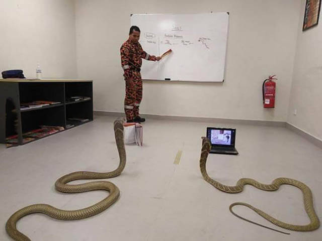
Teaching_Python.png, which looks like: and know where it is stored (you can rightclick > Save Image As...). (It will be convenient for you to have the image stored in the same directory as this workbook, so that you don't need relative paths - the notebook assumes you have done this).
Background
Image dimensions are measured in pixels - the image above has dimensions $640\times480$ pixels (width-height). Each pixel has an associated Red-Green-Blue (RBG) triple associated with it, which stores the relative shades of red, green, and blue at that pixel - giving the image color. (By contrast, a greyscale image only has one value per pixel which quantifies how dark that pixel is). As such, any $w\times h$ RGB image can be thought of as a $h\times w\times 3$ image-matrix or array of floating-point numbers, which allows us to manipulate images on a computer. Note that the order of $w$ and $h$ is changed as row-index is stored first in a 2D-array on a computer.
The SVD
The Singular Value Decomposition (SVD) of a matrix is a powerful theoretical tool and to a more modest degree, a useful computational tool too. For the purposes of these exercises we will introduce the SVD soley for use in image manipulation, however be aware that you will likely meet this (if you haven't already) at some point in the future and it has much more general interpretations.
Let $A\in\mathbb{R}^{m\times n}$ (a real $m\times n$ matrix), and let $K=\min\{n,m\}$. Then there exist orthogonal matrices $U\in\mathbb{R}^{m\times m}, V\in\mathbb{R}^{n\times n}$ and numbers $\sigma_{i}\in\mathbb{R}$ for each $i\in\{1,...,K\}$ ordered such that $\vert\sigma_{i}\vert\ge\vert\sigma_{i+1}\vert$ such that $A$ has the decomposition $$ \begin{align} A &= U\Sigma V^{\top} \\ \Sigma &= \mathrm{diag}\left(\sigma_{1}, ... , \sigma_{k} \right) \in\mathbb{R}^{m\times n}. \end{align} $$ We call $U$ the matrix of left-singular vectors and $V$ the matrix of right-sigular vectors (these vectors span the image space and domain space of $A$, respectively) and the $\sigma_{i}$ are the singular values. Note that $\Sigma$ is not necessarily square - it can be "tall" (has extra rows of zeros) or "long" (extra columns of zeros). This is formally a theorem and has a proof which we are not going to detail, because it's long and would require some theoretical setup which we thought we'd spare you from.
Some interpretation in the context of image-matrices:
- The larger singular values can be thought of as defining "large-scale" features, whereas the smaller singular values define sharp features in the image.
- For an image array, we have a SVD for each of the fixed-RGB slices through the array. I.e: We have a "red SVD", "green SVD" and "blue SVD" for each image.
- Due to the existance of machine precision (the smallest positive number that can be stored on a computer), small singular values may fall near or below this value and a computer cannot reliably work with these values. This is a big problem when trying to invert large systems and is central to the field of Inverse Problems.
- If we know the SVD, we know how to construct the image. We can use the SVD to change the image for better or worse if we want.
1 - Setup
Read in the image Teaching_Python using matplotlib's imread function, calling the output pythonPic.
This is a $64\times64\times3$ image-array.
Use matplotlib.pyplot.imshow and then matplotlib.pyplot.show to visualise the image.
NOTE: Read the above codeblock so that you know which names the various modules have been imported under!
Also store the dimensions in an array dims using the np.shape command.
Teaching_Python should look like the following image, possibly rescaled by matplotlib:
|
Image Noise Reduction (Greyscale)
Converting to Greyscale
We are now going to look at one of the uses for the SVD and low-rank approximations - filtering out noise from an image. Noise can arise in an image (or indeed, any data type) a number of ways, errors in communication, imprecisions when first storing the information, etc.
To prevent things from getting too complicated we are going to use a greyscale image to do this, so please run the following codeblock. This codeblock will provide you with:
- A new image,
monoPic, which is a greyscale version ofpythonPic - A function,
PlotGreyscale, which you may use to plot the greyscale images properly. CallingPlotGreyscale(image)will just plot the image arrayimage; if you give a second string argument such as byPlotGreyscale(image, 'Snazzy title'), your plot will also have the title 'Snazzy Title'. An example call is given in the codeblock.
def RGB2Gray(rgb):

    r, g, b = rgb[:,:,0], rgb[:,:,1], rgb[:,:,2]
    grey = 0.2989 * r + 0.5870 * g + 0.1140 * b

    return grey

def PlotGreyscale(img, titleStr=''):
    '''A function so that greyscale images plot correctly.
    Passing a second argument makes a title for the image.
    '''

    plt.title(titleStr)
    plt.imshow(img, cmap=plt.get_cmap('gray')) #Americanism...
    plt.show()

    return

monoPic = RGB2Gray(pythonPic)
PlotGreyscale(monoPic, 'Greyscale Picture')
